Analog IC application · Voltage encoded as pulse frequency

LM331: A Pulse Count Can Encode an Analog Voltage

Build the external network around one LM331, apply a small positive voltage and observe a changing pulse rate. Derive the charge-per-pulse equation, then see why a finite counting window, component tolerances and analog offsets keep a pulse count from being an automatically accurate voltage reading.

1. One converter, no microcontroller

The exact integrated circuit (IC) is Texas Instruments LM331N/NOPB in the P eight-pin plastic dual in-line package (PDIP). It is the commercial 0–70 °C variant, not an assumed LM231, LM331A or surface-mount substitute. Read the notch and pin-1 mark from above before wiring. The circuit uses a regulated 5.00 V bench supply, a separate low-voltage direct-current (DC) input source and a high-impedance oscilloscope or frequency counter. No microcontroller (MCU), firmware, mains connection or battery short-circuit experiment is required.

A voltage-to-frequency converter produces a pulse rate related to an input voltage. The LM331 does this through charge balance: a controlled current is switched for a nominally fixed interval, delivering a charge packet into an external capacitor. Between packets, a resistor removes charge. A larger input voltage requires more packets per second to maintain the balance. The digital-looking output does not remove the analog reference, resistor, capacitor, temperature and offset errors that set its scale.

The author reviewed the current manufacturer datasheet and executed the delivered host calculations and finite models. No IC was physically wired, no waveform was measured and no target program was executed. The figures and numbers below are source-based design expectations and constructed traces, not a tested instrument specification.

2. Trace all eight terminals and the external network

Units used below: Ω is ohm, kΩ is kilohm, µF is microfarad, nF is nanofarad, µA is microampere, µs is microsecond, mV is millivolt, nC is nanocoulomb, Hz is hertz and s is second.

PinNameThis fixture’s connection
1IOUT, switched current outputJoin Vx node at pin 6
2IREF, reference-current terminalRS = 14.0 kΩ to common ground, fixed 1% metal film
3FOUT, frequency output10 kΩ pull-up to +5 V and high-impedance instrument input
4GNDCommon return for supply, input source and instruments
5RC, timing terminalRT = 6.80 kΩ to +5 V; CT = 10.0 nF to ground
6THRESH, threshold inputVx, joined to pin 1 and the RL/CL network
7COMPIN, comparator inputVIN through RIN = 100 kΩ; CIN = 1 µF to ground
8VS, supplyRegulated +5.00 V, bypassed by 1 µF to ground at the IC

RL = 100 kΩ runs from Vx to a lower node Y. CL = 1 µF is in parallel with RL, between Vx and Y. A 47 Ω resistor runs from Y to common ground. That last resistor is important: it is the datasheet’s small hysteresis-producing branch, not a capacitor accidentally returned to a second supply. Omit the optional offset-adjustment injection shown in TI Figure 14; there is no negative rail in this fixture.

Use 1% metal-film RS, RL, RIN and RT; use a 5% 10 nF C0G/NP0 timing capacitor, whose stable ceramic dielectric suits timing. Use low-absorption polypropylene film for CL and CIN, each 1 µF, 5%, rated at least 16 V. The supply bypass can be a low-equivalent-series-resistance (ESR) 1 µF X7R ceramic rated at least 16 V. The 47 Ω and output pull-up resistors can be 5%, 0.25 W parts. All component ratings exceed this five-volt exercise; their tolerances still affect the result.

LM331N functional pin diagram shows pin 8 on regulated five volts with a one microfarad bypass, pin 4 on common ground, pin 7 fed through 100 kilohms with one microfarad input filter, pins 1 and 6 joined at Vx, parallel 100 kilohm RL and one microfarad CL from Vx to node Y, and 47 ohms from Y to ground. Pin 2 has 14 kilohms to ground. Pin 5 has 6.8 kilohms to five volts and ten nanofarads to ground. Pin 3 has a ten kilohm five-volt pull-up and a high-impedance scope output with common return.
External functional schematic based on TI Figure 14, adapted to 5 V and the restricted input range. Pin positions are grouped by function, not a top-view package drawing; numbers are the exact PDIP terminals. Editable Scalable Vector Graphics (SVG).

Power and source returns must actually meet at common ground. Connect an earth-referenced scope ground only to that return; never clip it to Vx or the timing terminal. The output is open collector: an internal transistor can pull FOUT down, while the external resistor supplies the rising level. A released output is high impedance, not an internally driven five-volt source. There is no light-emitting diode load or 50 Ω scope termination.

3. Restrict the experiment before calculating frequency

Use VIN only from 0.20 to 2.00 V and verify it with a DC voltmeter before connecting the source. The input source’s output must be referred to common ground and remain inside this range during changes. At VS = 5 V, the datasheet’s comparator common-mode upper limit is VS − 2 V, or 3 V; the selected input and expected small Vx ripple leave margin. Supply operation is specified from 4 to 40 V, but this is a five-volt experiment, not permission to test the 40 V boundary.

Set the supply current limit to 20 mA before connection. The LM331 table lists up to 6 mA at 5 V; the 10 kΩ output pull-up adds at most about 0.5 mA when LOW. Check actual current and terminal voltages; a current limit is not reverse-polarity protection. Keep all external instrument inputs high impedance and rated for a five-volt output. Do not connect FOUT directly to a 3.3 V microcontroller input.

TI Figure 14 uses a 15 V example and optional gain/offset adjustments. This fixture deliberately narrows the input, uses a fixed RS and selects the permitted 1 µF CIN to match the approximately 0.1 s RL×CL time constant. The datasheet’s advertised linearity and the Figure 14 typical curve are not guaranteed accuracy for this adaptation. Offset trimming, gain calibration, component behavior, loading and a physical validation remain unfinished bench work.

4. Derive the nominal charge balance

The application model uses reference current I ≈ 1.90 V / RS. With RS = 14,000 Ω, I ≈ 135.714 µA. The nominal one-shot interval is tON ≈ 1.1 RT CT = 1.1 × 6800 × 10 nF = 74.8 µs. One current packet carries Q = I × tON ≈ 10.1514 nC. A one-shot is a circuit that holds a temporary state for a timing interval after a trigger.

In average balance, packet current Q × f approximately equals VIN/RL. Therefore f ≈ VIN/(RL Q), or equivalently:

fOUT ≈ (VIN / 2.09 V) × (RS / RL) × 1/(RT CT)
For the selected nominal parts: 985.083 Hz per volt
VIN = 0.20 V → about 197.017 Hz
VIN = 1.00 V → about 985.083 Hz
VIN = 2.00 V → about 1970.166 Hz

The 2.09 V constant is the nominal 1.90 V reference multiplied by the nominal 1.1 timing factor. It is not a precision external reference supplied by the program. At 2 V, the nominal pulse duty is about 0.1474, well below continuous current injection. Duty is the fraction of a cycle spent in the active pulse. The ideal full-current overload boundary is outside the lesson’s permitted input and must not be explored by increasing VIN.

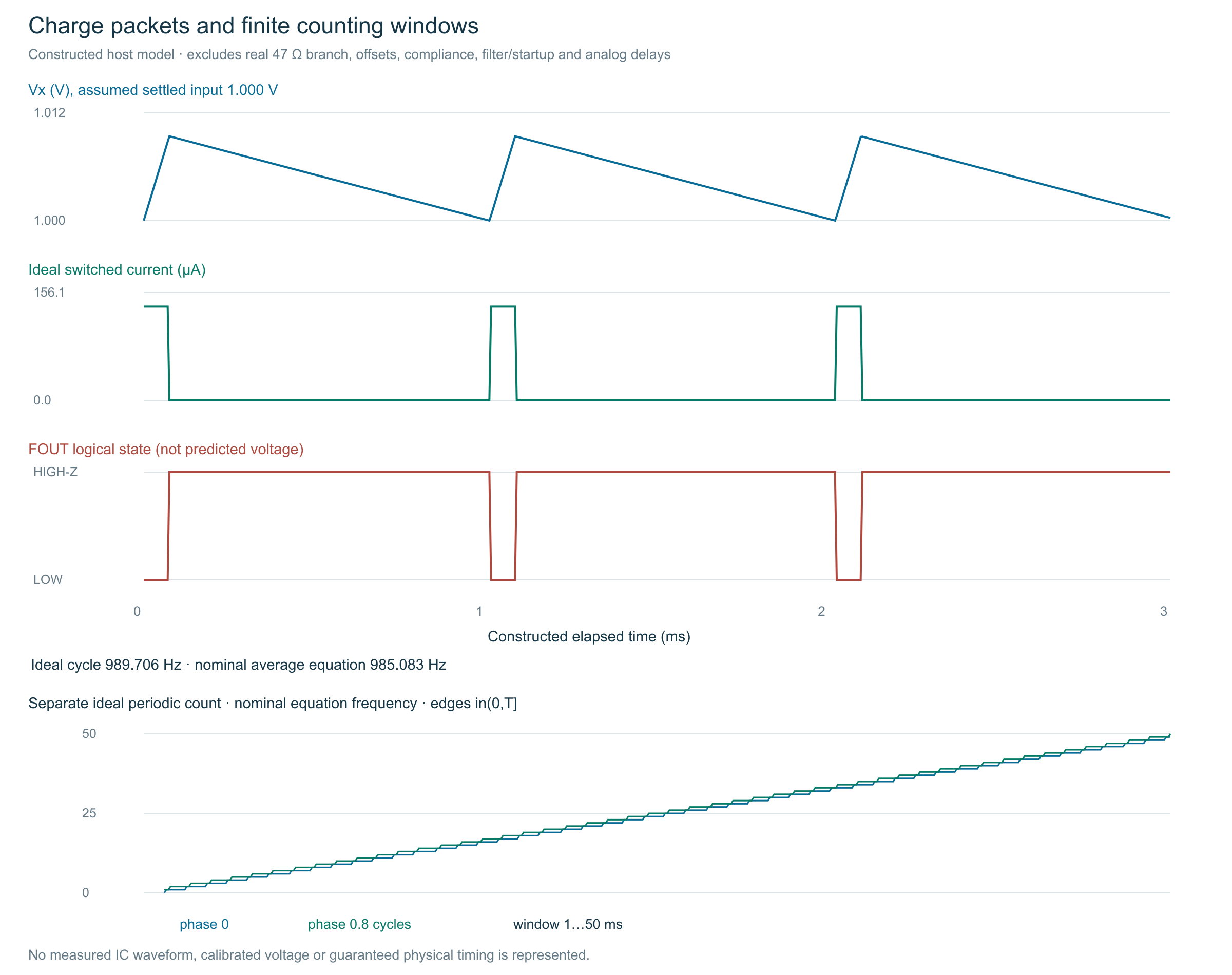
For perspective, a packet divided by CL suggests a roughly 10 mV voltage step before accounting for discharge during the pulse. The 47 Ω branch also adds a small immediate voltage change from current. These effects, comparator offset, leakage and current-source behavior mean the real Vx waveform is not obtained by drawing an exact 10 mV staircase. The supplied model explicitly omits the 47 Ω branch and analog nonidealities rather than pretending to simulate the physical IC.

5. A counting window adds another boundary

A counter that observes N qualifying edges during a measured window T reports N/T. At T = 0.1 s, one count is 10 Hz, or about 10.151 mV using the nominal scale. At one second, one count is 1 Hz, or about 1.015 mV. A longer window reduces this count granularity, but it does not fix gain error, drift, offset, missed edges or a wrong timebase.

The ideal periodic counter uses edges in the interval (0, T]: it excludes an edge exactly at the start and includes one exactly at the end. Changing the starting phase can change the ideal count by one. The program’s one-count voltage value is resolution under the nominal conversion scale, not a complete uncertainty interval. An actual frequency counter can have its own gate behavior, trigger thresholds and timebase error.

No edges is especially ambiguous. It can mean a low input, startup or overload, absent power, disconnected output, failed pull-up or a counter problem. TI describes an overload condition in which the current source stays on and the frequency becomes zero. The program labels a user-entered zero count as NO_EDGES_NOT_PROOF_OF_ZERO. Its nominal arithmetic voltage field is zero when the entered count is zero, but that number is not a measured-zero conclusion: the status explicitly refuses that interpretation.

Constructed ideal RC trace at one volt shows Vx rising during nominal 74.8 microsecond current packets and decaying between them, the switched current and logical FOUT LOW intervals. A separate ideal counting-window plot shows two start phases producing staircase counts around the nominal frequency times window. The model excludes the real 47 ohm hysteresis branch and analog errors.
Exact segments of a simplified ideal current-source/RL/CL model and a separate nominal periodic edge counter. The physical 47 Ω branch, offsets, startup and compliance are excluded; no measured waveform. Editable SVG.

6. Complete host calculator and finite model

The supplied Python program evaluates the primary nominal equation, passive-component corners, a simplified cycle and finite-window counts. It uses exact exponential RC segments in that simplified model: during the packet CL charges toward I×RL; afterward it decays through RL until Vx returns to the assumed settled input threshold. This model’s average Vx is slightly above VIN, so its frequency differs from the simple VIN/RL approximation. That discrepancy illustrates the model boundary; it is not a correction calibrated for a real LM331.

The passive corners enumerate 16 combinations of RS/RL/RT at ±1% and CT at ±5%. At 1 V they span approximately 910.492–1068.563 Hz. This excludes the IC’s own reference/gain/offset and every physical uncertainty, so do not label it a total accuracy bound. The code rejects non-finite values and restricts component, voltage, time and count domains before arithmetic.

Complete lm331_window.py
"""HOST-ONLY LM331 nominal charge arithmetic and finite counting model.

TI SNOSBI2C Figure14 external network adapted to 5.0V/0.2..2.0V.
Not SPICE, not silicon/bench validation, no GPIO or target firmware.
"""
import argparse
import itertools
import json
import math

RS, RL, RT, CT, CL = 14000.0, 100000.0, 6800.0, 1e-8, 1e-6


def number(x, low, high, name):
    if type(x) not in (int, float) or not math.isfinite(x) or not low <= x <= high:
        raise ValueError(name)
    return float(x)


def nominal(vin, rs=RS, rl=RL, rt=RT, ct=CT):
    vin = number(vin, .2, 2, 'VIN_0_2_TO_2V')
    rs = number(rs, 12000, 17000, 'RS')
    rl = number(rl, 90000, 110000, 'RL')
    rt = number(rt, 6000, 7500, 'RT')
    ct = number(ct, 8e-9, 12e-9, 'CT')
    current = 1.90 / rs
    pulse = 1.1 * rt * ct
    charge = current * pulse
    frequency = vin / (rl * charge)
    duty = frequency * pulse
    if not all(math.isfinite(x) and x > 0 for x in (current, pulse, charge, frequency, duty)) or duty >= .25:
        raise ValueError('MODEL_RANGE')
    return {'vin_V': vin, 'reference_current_A_nominal': current,
            'pulse_s_nominal': pulse, 'charge_C_nominal': charge,
            'frequency_Hz_nominal': frequency, 'duty_nominal': duty,
            'scale_Hz_per_V_nominal': frequency / vin}


def count_periodic(frequency, window, phase=0):
    """Ideal periodic edges in (0,T], phase = fractional cycle at t=0."""
    f = number(frequency, .01, 100000, 'FREQUENCY')
    t = number(window, .001, 60, 'WINDOW')
    phase = number(phase, 0, .999999999, 'PHASE')
    return math.floor(f * t + phase) - math.floor(phase)


def infer_count(count, window, vin_for_scale=1):
    if type(count) is not int or not 0 <= count <= 10000000:
        raise ValueError('INTEGER_COUNT')
    window = number(window, .001, 60, 'WINDOW')
    k = nominal(vin_for_scale)['scale_Hz_per_V_nominal']
    return {'observed_count': count, 'window_s': window,
            'count_rate_Hz': count / window,
            'voltage_V_from_nominal_scale': count / window / k,
            'one_count_Hz': 1 / window,
            'one_count_V_nominal': 1 / window / k,
            'status': 'NO_EDGES_NOT_PROOF_OF_ZERO' if count == 0 else 'COUNT_ONLY_NOT_CALIBRATED_VOLTAGE'}


def passive_corners(vin):
    values = [nominal(vin, RS * s, RL * l, RT * t, CT * c)['frequency_Hz_nominal']
              for s, l, t, c in itertools.product((.99, 1.01), (.99, 1.01), (.99, 1.01), (.95, 1.05))]
    return {'minimum_Hz': min(values), 'maximum_Hz': max(values),
            'scope': 'Passive RS/RL/RT1percent and CT5percent only; excludes IC gain/offset, temperature, leakage, calibration and timing instrumentation.'}


def ideal_cycle(vin):
    """Exact RC segments of a simplified ideal source/CL/RL model.

    Excludes physical R47 hysteresis branch, comparator/timer delays, reference
    tolerance, source compliance, capacitor parasitics, startup and input filter.
    Starts at an assumed settled trigger threshold Vx=Vin.
    """
    n = nominal(vin)
    current, on = n['reference_current_A_nominal'], n['pulse_s_nominal']
    tau, asymptote = RL * CL, current * RL
    peak = asymptote + (vin - asymptote) * math.exp(-on / tau)
    off = tau * math.log(peak / vin)
    period = on + off
    return {'on_s': on, 'off_s': off, 'period_s': period,
            'frequency_Hz_ideal_RC': 1 / period, 'peak_V_ideal': peak,
            'ripple_V_ideal': peak - vin, 'threshold_V': vin}


def trace(vin=1, duration=.003, step=.000005):
    duration = number(duration, .0001, .02, 'DURATION')
    step = number(step, .000001, .00002, 'STEP')
    if duration / step > 20000:
        raise ValueError('TRACE_LIMIT')
    n, cycle = nominal(vin), ideal_cycle(vin)
    rows = []
    for i in range(int(duration / step) + 1):
        t = i * step
        phase = t % cycle['period_s']
        active = phase < cycle['on_s']
        if active:
            end = n['reference_current_A_nominal'] * RL
            vx = end + (vin - end) * math.exp(-phase / (RL * CL))
        else:
            vx = cycle['peak_V_ideal'] * math.exp(-(phase - cycle['on_s']) / (RL * CL))
        rows.append({'t_s': t, 'vx_V': vx, 'pump_A': n['reference_current_A_nominal'] if active else 0,
                     'FOUT_model': 'LOW' if active else 'RELEASED_HIGH_Z'})
    return rows


def report(vin=1, window=.1, count=None):
    n = nominal(vin)
    if count is None:
        count = count_periodic(n['frequency_Hz_nominal'], window)
        origin = 'CONSTRUCTED_PERIODIC_COUNT_NOT_MEASURED'
    else:
        origin = 'USER_ENTERED_COUNT_NOT_HARDWARE_VALIDATED'
    return {'nominal': n, 'passive_corners': passive_corners(vin),
            'ideal_cycle': ideal_cycle(vin), 'count': infer_count(count, window),
            'count_origin': origin, 'hardware_tested': False, 'target_executed': False}


if __name__ == '__main__':
    p = argparse.ArgumentParser(description=__doc__)
    p.add_argument('--vin', type=float, default=1)
    p.add_argument('--window', type=float, default=.1)
    p.add_argument('--count', type=int, default=None)
    a = p.parse_args()
    print(json.dumps(report(a.vin, a.window, a.count), indent=2))

Complete host calculator/model · Blank bench worksheet · Code and reproducible tests ZIP

python lm331_window.py --vin 1 --window 0.1
# Enter a count you actually observed, without relabelling it as calibrated:
python lm331_window.py --vin 1 --window 0.1 --count 98
python -B test_lm331.py

7. Build and observe without assuming success

  1. With power off, identify LM331N/NOPB and its notch. Check each numbered terminal against the functional schematic. Measure the fixed resistors; check that CL and RL share Vx and Y, and that Y reaches ground only through the 47 Ω branch.
  2. Keep the input source disconnected while verifying its 0.20 V starting output and common-return arrangement. Verify the main supply is 5.00 V with a 20 mA limit. Connect supply, bypass and ground with short leads.
  3. Power up and check VS at pin 8, ground at pin 4 and the reference terminal near its expected value without loading it significantly. If a value or current is wrong, switch off and inspect wiring. Do not search for a frequency by increasing the supply or input.
  4. Connect the prechecked input through RIN. Use high-impedance instruments. Record actual VIN at the source and filtered pin 7, Vx at pin 6, output LOW/HIGH levels and pulse timing. Wait at least one second after a change as a conservative initial filter-settling allowance; verify stability rather than treating that wait as a proven settling guarantee.
  5. Compare 0.20, 0.50, 1.00 and 2.00 V. Count falling edges consistently over 0.1 s and one second. Preserve the actual gate duration, trigger setup and counter model. The worksheet has no measured rows because the author did not perform this bench run.
  6. Before removing the 5 V supply, set the separate input source to 0 V, verify that the filtered pin-7 voltage has returned near zero, then disconnect its positive lead while retaining the common return. Do not leave a positive input driving an unpowered LM331: the absolute input limit tracks +VS. Do not inject out-of-range voltages as a fault test. Use the supplied finite numerical cases for error behavior instead; they are not evidence of physical overload recovery.

8. What was checked and what remains

The author’s 26 host groups execute the delivered program: equation equivalence, packet charge balance, input scaling, timing/component dependence, duty margin, finite-range rejection, half-open counting boundaries, phase ambiguity, zero-count status, passive corners, exact simplified RC endpoints and charge conservation, trace limits and the actual command-line output. Package checks are separate. No hardware, firmware compilation or target execution is claimed.

Keep nominal source arithmetic distinct from measured accuracy. The basic stand-alone circuit has comparator offset and finite ripple; TI’s precision op-amp circuit is a different topology. Do not silently claim its specifications here. Read the electronics course for circuit fundamentals and Circuitpedia for component terms before wiring a new package.

9. Challenge: is a longer gate a calibration?

At nominal one volt, your one-second count is repeatable but consistently lower than the equation. Would counting for ten seconds establish that the input is correct?

Answer

No. A longer gate can reduce one-count granularity relative to the total, while a scale error, reference error, offset, loading error or wrong timebase remains. Verify input and setup, quantify uncertainty and calibrate the actual circuit if needed. Repeatability is not accuracy, and a zero count is not proof of a zero input.

10. Current primary reference