
One knob can move two electrical controls together. Use a Bourns PDB182 to measure both output voltages at the same shaft positions. First read both wipers with a high-impedance meter alone. Then connect one 10 kΩ load to gang A, move it to gang B, and remove it again. The shared shaft stays at the same mark for those four readings. A change that follows the resistor shows what the load adds to any baseline difference.
A potentiometer is a resistive strip with a movable contact called the wiper. When the strip ends connect to a fixed voltage and its return, the wiper taps a fraction of that voltage. Each gang is one independent strip and wiper. A dual-gang part moves both wipers with one shaft. Tracking here means how closely those two voltage fractions agree at a given shaft position. Taper is the shape of the ratio-versus-position curve for one gang.
This is a proposed bench experiment. The worked rows are constructed to explain the arithmetic. Fill the blank worksheet with your own readings.
Identify the part and its terminal rows
Use the exact Bourns PDB182-K420K-103B1. The Bourns ordering table identifies a dual section, vertical down-facing K terminals, detent option 4 for no detents, 20 mm shaft length, and K for the knurled shaft. Code 103 denotes 10 kΩ nominal per strip. Suffix B1 selects the curve labeled (1B) in the B-series chart. The chart separately identifies B3 as the default for a dual-gang order with an unsuffixed B taper. Keep the B1 suffix in your notes. The taper chart describes the curve, while this bench measures one specimen’s agreement between gangs.
The current series sheet gives a ±20% standard total-resistance tolerance at 10 kΩ and a 300° ±5° mechanical angle. The tolerance applies between the fixed ends. Two strips can have different end-to-end resistance and still tap the same voltage fraction. Their wipers can also disagree even if the totals match. The cited sources give no numerical gang-tracking acceptance limit for this exact orderable. Use the repeat readings and meter uncertainty when interpreting a difference.
Face the shaft with the downward terminal rows below it. In the PDB182-K drawing, the row nearest the shaft is R1 (gang A here) and the row behind it is R2 (gang B). The view numbers the three positions 1, 2, and 3 from left to right. The separate schematic marks the R2 equivalents 1′, 2′, and 3′. Mark the two rows before turning the assembly over. Numbering reverses if you view the assembly from the opposite side.
With the part completely disconnected, measure 1–3 and 1′–3′ and record the two totals. As the shaft turns, the resistance from each center terminal to one end should rise while its resistance to the other end falls. At the counterclockwise stop (CCW), check for a low resistance from 1 to 2 and from 1′ to 2′. At the clockwise stop (CW), check the corresponding paths to 3 and 3′. The endpoint resistance can be finite. Check that the two gangs remain separate before wiring their supply ends together. Resolve a reversed, intermittent or ambiguous terminal reading before applying power.
Build the divider and movable load
- The exact six-terminal potentiometer, its panel nut, a shaft pointer and a printed angle scale. Mount it so pulling a clip does not move the body or turn the shaft.
- A regulated 3.00 V direct-current supply (DC) with a 5 mA current limit. Use a low-voltage bench source and insulated test leads.
- One 10 kΩ, 1%, ¼ W resistor with insulated clips. Measure its actual resistance before fitting it. Keep one end on the common return. Its other end selects A, B or a parked position insulated from the circuit.
- One battery-powered Fluke 87V MAX digital multimeter. Keep the black lead in COM, its common terminal, and the red lead in the voltage/resistance jack. Measure loose resistors only with power removed. Use the 6.000 V DC range for powered readings. A second matching meter is optional if its input loading is recorded.
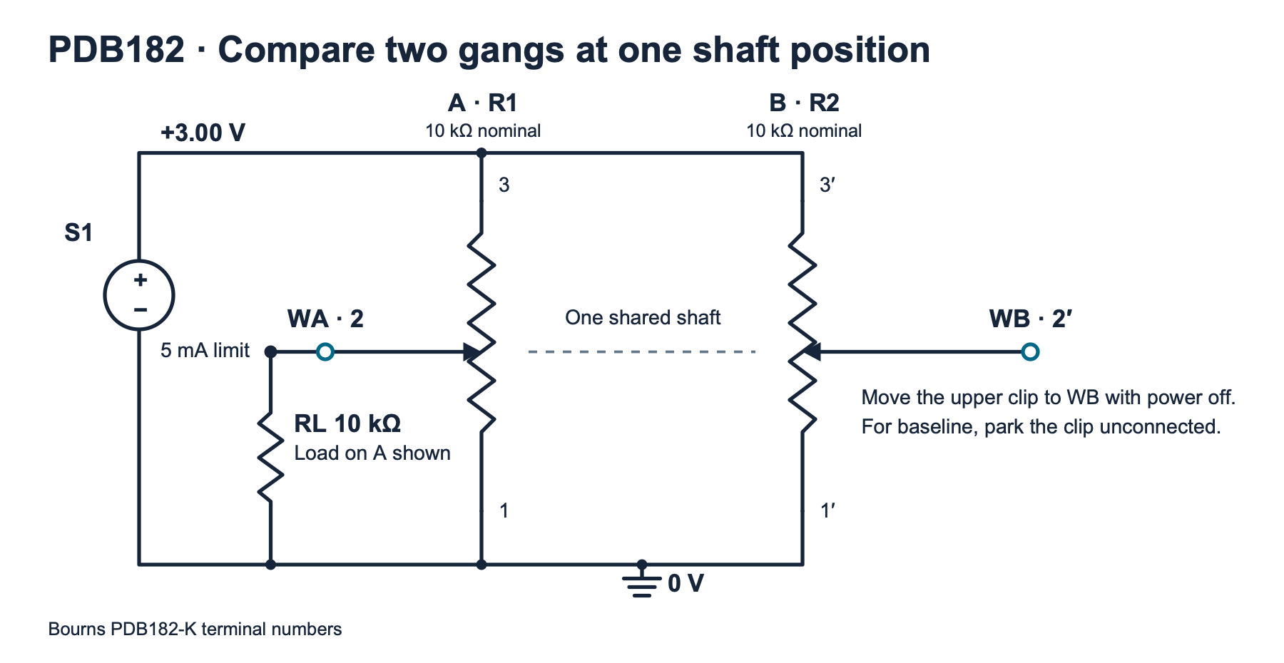
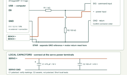
fixture.svg)| Terminals | Connection |
|---|---|
| A3 and B3′ | S1 positive, 3.00 V. Measure the supply here for every condition. |
| A1 and B1′ | S1 negative, the meter reference and the load resistor’s lower end. |
| A2 and B2′ | Separate voltage test points WA and WB. Move the single resistor’s upper clip to only one wiper during a loaded reading. |
At 3.10 V, two 8 kΩ tracks can each draw about 0.39 mA without the extra load. A 9.8 kΩ load can add at most about 0.32 mA. These conservative bounds put the whole fixture near or below 1.1 mA, or about 3.4 mW from the source. They assume correctly identified terminals and the planned resistance range. If the source reaches its 5 mA limit, power off and look for a miswire or clip short. Keep all connections within this low-voltage experiment.
Measure four conditions at each shaft mark
- Use the pointer and angle scale to mark both gentle mechanical stops. Measure the actual span and divide it into positions at 10%, 30%, 50%, 70% and 90%. At a 300° span, for example, the 30% mark is 90° from the CCW stop. These are fractions of shaft travel. Use the actual wiper voltage to determine the electrical ratio at each mark.
- With the load clip parked, power on and check the rail. Move toward the first mark from the CCW side. Avoid overshooting. If you pass a mark, back up and approach it again from the same direction. Mark or secure the shaft without forcing it. The no-detent shaft can move slightly while you work with clips.
- Measure the common supply, WA, and WB, with the meter’s black lead fixed at the return. Keep the shaft stationary while moving the red lead. Enter the three voltages as
baseline. The meter is the remaining load in this condition. - Turn the supply off. Without moving the shaft, place the upper load clip on WA. Power on, let the reading settle and remeasure the supply and both wipers. Record
load_a. With power off again, move that same clip to WB, power up and recordload_b. Keep both wiper wires separate throughout. - Power down and park the upper clip. Restore power and record
repeatat the same mark. Check that the pointer and readings have returned. If they have shifted, look for motion or a connection problem and repeat the four-condition set. Proceed to the next mark from the same direction.
The unloaded gang in each loaded run serves as a control. Its normalized ratio should be close to its baseline within the setup’s repeatability. If both move when only one is loaded, check for shaft motion, shared return resistance, a supply leaving regulation or an accidental link between wipers. Normalize each reading to its own measured supply to remove the first-order effect of small rail changes. A shifting reference or moving shaft needs a new set of observations.
Separate tracking from a change caused by the load
Divide each wiper voltage by that row’s supply voltage to get a fraction. For example, 1.53 V at a 3.00 V supply gives 0.51, or 51%. Subtract the B baseline percentage from the A baseline percentage. The result is a signed difference in percentage points, abbreviated pp in the output. A baseline of 51% versus 49% gives +2 pp. That difference describes the two ratios directly.
At one shaft position, call the resistance above a wiper Rtop and the resistance below it Rbottom. The ideal meter-only ratio x is approximately Rbottom ÷ (Rtop + Rbottom). Connecting the external resistor to ground puts it in parallel with the bottom portion. The two branches share the same voltage and provide a lower combined resistance. The tapped voltage then falls.
For a prediction, use the measured baseline ratio as x and the measured end-to-end resistance as RT. The Thévenin equivalent represents the divider at the wiper as a voltage source with a series resistance. Its source voltage is xVS and the series resistance is RTx(1 − x). With the measured load RL, the predicted loaded ratio is xRL ÷ [RL + RTx(1 − x)]. This approximation treats the supply as stiff and the wiper contact resistance as negligible. It uses the observed ratio rather than assuming a taper.
At an illustrative electrical ratio of 0.50 with a 10 kΩ strip, each portion is 5 kΩ. The equivalent resistance is 2.5 kΩ. A 10 kΩ load gives 0.40, a change of −10 pp or −0.30 V at 3.00 V. At a mechanical 50% mark, use the observed ratio for each gang. The same load can cause unequal shifts if the two baseline fractions or track totals differ.
| Condition | A voltage | B voltage |
|---|---|---|
| Baseline | 1.530 V | 1.470 V |
| Load A | 1.224 V | 1.470 V |
| Load B | 1.530 V | 1.176 V |
| Repeat | 1.533 V | 1.467 V |
The example gives +2.0 pp at baseline, an A load shift of −10.2 pp, and a B load shift of −9.8 pp. The unloaded controls stay at their original ratios. The repeat rows differ by +0.1 pp and −0.1 pp. Treat this exercise as an arithmetic example. For real observations, report the range of baseline differences across your five marks and how large the repeat variation was. A much larger change that follows the load supports a loading explanation for that part of the mismatch.
The 87V MAX has a nominal 10 MΩ voltage input. With a 12 kΩ track the maximum ideal equivalent resistance is 3 kΩ, so the meter alone can reduce the ratio by up to about 0.03% of its value in this model. Its DC voltage accuracy on the 6.000 V range is ±(0.05% of reading + one count) under Fluke’s specified conditions. At 1.5 V this is about ±1.75 mV for one reading. Counts are steps of the least significant displayed digit. Include the supply reading, meter repeatability and shaft placement in your comparison. Near an end stop a small absolute voltage error can dominate a small apparent mismatch.
Compare the four runs with the complete program
Fill a copy of the blank worksheet (ZIP: observations-blank.csv). Keep one row for each of baseline, load_a, load_b and repeat at every position used. Enter the mechanical mark in position_pct, the case in condition, and the three voltages in supply_v, wiper_a_v and wiper_b_v. Remove unused starter sets. Keep a separate note of the meter, direction and measured resistor values.
Save the code below as tracking.py and use Python 3.9 or later. Run python3 tracking.py observations.csv --track-a 10000 --track-b 10000 --load 10000, replacing those example resistance values with your measured ohms. To reproduce the table use constructed-examples.csv (ZIP: constructed-examples.csv) and the shown example resistance values. Output is comma-separated values (CSV) printed to the terminal. The model columns predict the changes for A and B, while the control columns show what happened to the other gang. The repeat columns expose movement or measurement drift after removing the load.
The program rejects incomplete or duplicated cases, out-of-range readings, invalid resistance arguments and malformed files. It expects a rail between 2.90 V and 3.10 V, nonnegative wiper readings within the measured supply rail, measured track totals between 7,800 Ω and 12,200 Ω, and a measured load between 9,800 Ω and 10,200 Ω. These are worksheet scope checks. Resolve any row error at the bench before calculating again. Printed decimals describe arithmetic precision. Decide which differences are resolved from your observed variation and instrument limits.
"""Compare two wiper ratios at each shaft position and quantify load shifts."""
import argparse
import csv
import math
from pathlib import Path
import sys

HEADER = ("position_pct", "condition", "supply_v", "wiper_a_v", "wiper_b_v")
CONDITIONS = ("baseline", "load_a", "load_b", "repeat")
OUTPUT = (
    "position_pct", "baseline_a_pct", "baseline_b_pct", "baseline_a_minus_b_pp",
    "a_load_shift_pp", "b_load_shift_pp", "b_control_shift_pp", "a_control_shift_pp",
    "a_model_shift_pp", "b_model_shift_pp", "repeat_a_shift_pp", "repeat_b_shift_pp",
)


def number(row, key):
    raw = row[key]
    if raw is None or not raw.strip():
        raise ValueError(f"{key} is required")
    try:
        value = float(raw)
    except ValueError:
        raise ValueError(f"{key} must be a number") from None
    if not math.isfinite(value):
        raise ValueError(f"{key} must be finite")
    return value


def read_groups(stream):
    reader = csv.DictReader(stream, strict=True)
    if reader.fieldnames != list(HEADER):
        raise ValueError("CSV header must be " + ",".join(HEADER))
    groups = {}
    for row in reader:
        try:
            if None in row:
                raise ValueError("too many columns")
            position = number(row, "position_pct")
            supply = number(row, "supply_v")
            a = number(row, "wiper_a_v")
            b = number(row, "wiper_b_v")
            condition = row["condition"]
            if not 0 <= position <= 100:
                raise ValueError("position_pct must be within 0–100")
            if not 2.90 <= supply <= 3.10:
                raise ValueError("supply_v must be within 2.90–3.10 V")
            if not (0 <= a <= supply and 0 <= b <= supply):
                raise ValueError("wiper voltages must stay within the measured rail")
            if condition not in CONDITIONS:
                raise ValueError("unknown condition")
            group = groups.setdefault(position, {})
            if condition in group:
                raise ValueError(f"duplicate {condition} for position {position:g}")
            group[condition] = (a / supply, b / supply)
        except ValueError as exc:
            raise ValueError(f"row {reader.line_num}: {exc}") from exc
    if not groups:
        raise ValueError("supply at least one observation")
    return groups


def model_shift(fraction, track_ohm, load_ohm):
    equivalent_ohm = track_ohm * fraction * (1 - fraction)
    loaded = fraction * load_ohm / (load_ohm + equivalent_ohm)
    return loaded - fraction


def summarize(groups, track_a, track_b, load):
    rows = []
    for position, group in sorted(groups.items()):
        missing = [name for name in CONDITIONS if name not in group]
        if missing:
            raise ValueError(f"position {position:g}: missing {', '.join(missing)}")
        a, b = group["baseline"]
        a_loaded, b_control = group["load_a"]
        a_control, b_loaded = group["load_b"]
        a_repeat, b_repeat = group["repeat"]
        values = (
            a, b, a - b, a_loaded - a, b_loaded - b,
            b_control - b, a_control - a,
            model_shift(a, track_a, load), model_shift(b, track_b, load),
            a_repeat - a, b_repeat - b,
        )
        rows.append([f"{position:g}", *(f"{100 * value:.3f}" for value in values)])
    return rows


def main():
    parser = argparse.ArgumentParser(description=__doc__)
    parser.add_argument("sheet", help="worksheet CSV path or - for standard input")
    parser.add_argument("--track-a", type=float, required=True, help="A end-to-end ohms")
    parser.add_argument("--track-b", type=float, required=True, help="B end-to-end ohms")
    parser.add_argument("--load", type=float, required=True, help="single load in ohms")
    args = parser.parse_args()
    try:
        for option, value in (("--track-a", args.track_a), ("--track-b", args.track_b)):
            if not 7800 <= value <= 12200:
                raise ValueError(f"{option} must be within 7800–12200 Ω")
        if not 9800 <= args.load <= 10200:
            raise ValueError("--load must be within 9800–10200 Ω")
        if args.sheet == "-":
            groups = read_groups(sys.stdin)
        else:
            with Path(args.sheet).open(encoding="utf-8-sig", newline="") as stream:
                groups = read_groups(stream)
        rows = summarize(groups, args.track_a, args.track_b, args.load)
    except (OSError, UnicodeError, csv.Error, ValueError) as exc:
        parser.exit(2, f"{exc}\n")
    writer = csv.writer(sys.stdout, lineterminator="\n")
    writer.writerow(OUTPUT)
    writer.writerows(rows)


if __name__ == "__main__":
    main()
Trace a difference before attributing it
- A rises as B falls. Check which fixed end is positive on each row. Compare the actual shaft-side view with the printed drawing and verify both wipers with the disconnected resistance test.
- The loaded ratio barely changes. Check the clip’s lower return and measure the resistor with power off. Repeat at a midrange electrical ratio, where the divider’s equivalent resistance can be larger than at an endpoint.
- The baseline repeat changes too. Inspect the shaft mark, the mounting nut and the clip connections. Correct the mechanical or wiring problem and reacquire the complete set.
- A stable difference stays with one gang. Compare its repeat readings and verify by exchanging meter channels if you used two meters. A persistent baseline difference is an observation about this specimen and fixture. An acceptance limit for a stereo control would depend on the intended use and its manufacturer specification.
The general potentiometer lesson explains the single-strip divider and common uses. Potentiometers: A Quick Overview
Challenge
Two ideal gangs both tap 60% of their supply with the meter alone. One has an 8 kΩ track and the other has a 12 kΩ track. What ratios do you predict if you clip the same 10 kΩ load onto each in turn? What should happen to the unloaded gang in either run?
Check your answer
The equivalent resistances are 8,000 × 0.6 × 0.4 = 1,920 Ω and 12,000 × 0.6 × 0.4 = 2,880 Ω. The loaded ratios are about 50.34% and 46.58%. The other gang stays near its own 60% baseline with an ideal shared supply and no shaft movement. The experiment can therefore show excellent baseline tracking alongside different loaded responses.
Primary references and downloads
- Bourns PDB18 series data sheet, Rev. 05/26. Page 1 gives the series ratings, page 3 shows the PDB182-K dual-gang terminals, and page 5 gives the ordering fields and B1 curve.
- Bourns product change notification K1922A. Page 37 lists PDB182-K420K-103B1 among affected order quantities. Use this to identify the exact orderable.
- Fluke 87V MAX users manual, Rev. 1. Printed pages 10–11 describe voltage measurements and loading. Pages 41 and 45 list DC accuracy and voltage input impedance.
Download the experiment files (ZIP) (ZIP: experiment-tests-v1.zip). Includes the full Python program, tests, blank worksheet, constructed example, original SVG and full-size PNG.
Download the complete reader files (ZIP): the original editable drawing, PNG, worksheet and code in pdb182-dual-gang-tracking-load. The full main program is also included above.