
Two capacitors in series can divide a voltage one way just after switch-on and another way after settling. Build a 5 V fixture with two film capacitors and a resistor across each. Capture the supply node and the midpoint together. Then change only the lower resistor and see which part of the trace should move.
Build the low-voltage fixture
A shunt is a parallel path across a component. Here the resistors carry a small direct current (DC) and set the long-time midpoint. The capacitors remain in place for both runs. Use the specified nonpolar metallized polyester film parts, which can be installed either way round in this fixture. These exact order codes specify ±10% capacitance tolerance and 63 V DC. Keep the entire experiment at 5 V and use no charged capacitor bank or mains-connected circuit.
| Part | Value | Connections |
|---|---|---|
| C1 | 2.2 µF, Vishay MKT1820522065, 10 mm lead pitch | VIN to MID |
| C2 | 4.7 µF, Vishay MKT1820547065, 15 mm lead pitch | MID to 0 V |
| R1 | 47 kΩ, 1% metal film | VIN to MID, across C1 |
| R2 | 100 kΩ in A, 47 kΩ in B, 1% metal film | MID to 0 V, across C2 |
| R3 | 1 kΩ, 0.25 W | After the series switch, before VIN |
| S1 | Single-pole single-throw (SPST) switch | Supply positive to R3 |
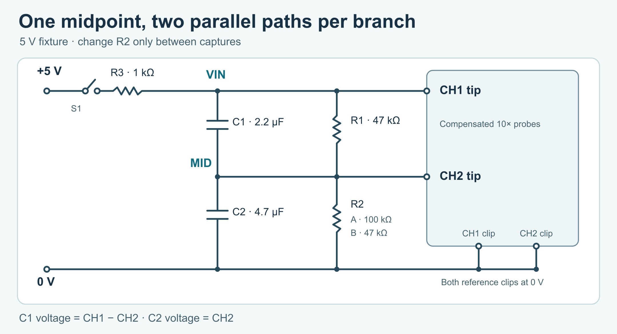
tricky-circuit-campaigns133-138/batch-014/packages/series-capacitor-voltage-sharing/functional.svg).Use a current-limited 5.0 V bench supply with an isolated low-voltage output. Set its limit around 20 mA. R3 limits the initial or short-circuit current to roughly 5 mA at the nominal supply, even if the current-limit response is slow. Its nominal short-circuit dissipation is 25 mW. The resistor and the series capacitance also slow the applied edge. The analyzer uses VIN measured after R3, so it can follow that real input rather than treating the bench supply setting as the waveform.
Use two compensated Tektronix P2220 passive probes at 10× on compatible 1 MΩ oscilloscope inputs, or a checked equivalent with the same modeled resistance. Set the matching attenuation in the scope and use DC coupling. The P2220 specifies 10 MΩ at 10×, with 13–17 pF input capacitance in its instructions. Connect the supply negative and both scope reference clips only to fixture 0 V. Put the first tip on VIN and the second on MID. Connecting a grounded reference clip to MID would short the lower branch. If you want the voltage across C1, subtract the second channel from the first. C2 is the second channel directly.
Separate the fast and slow limits
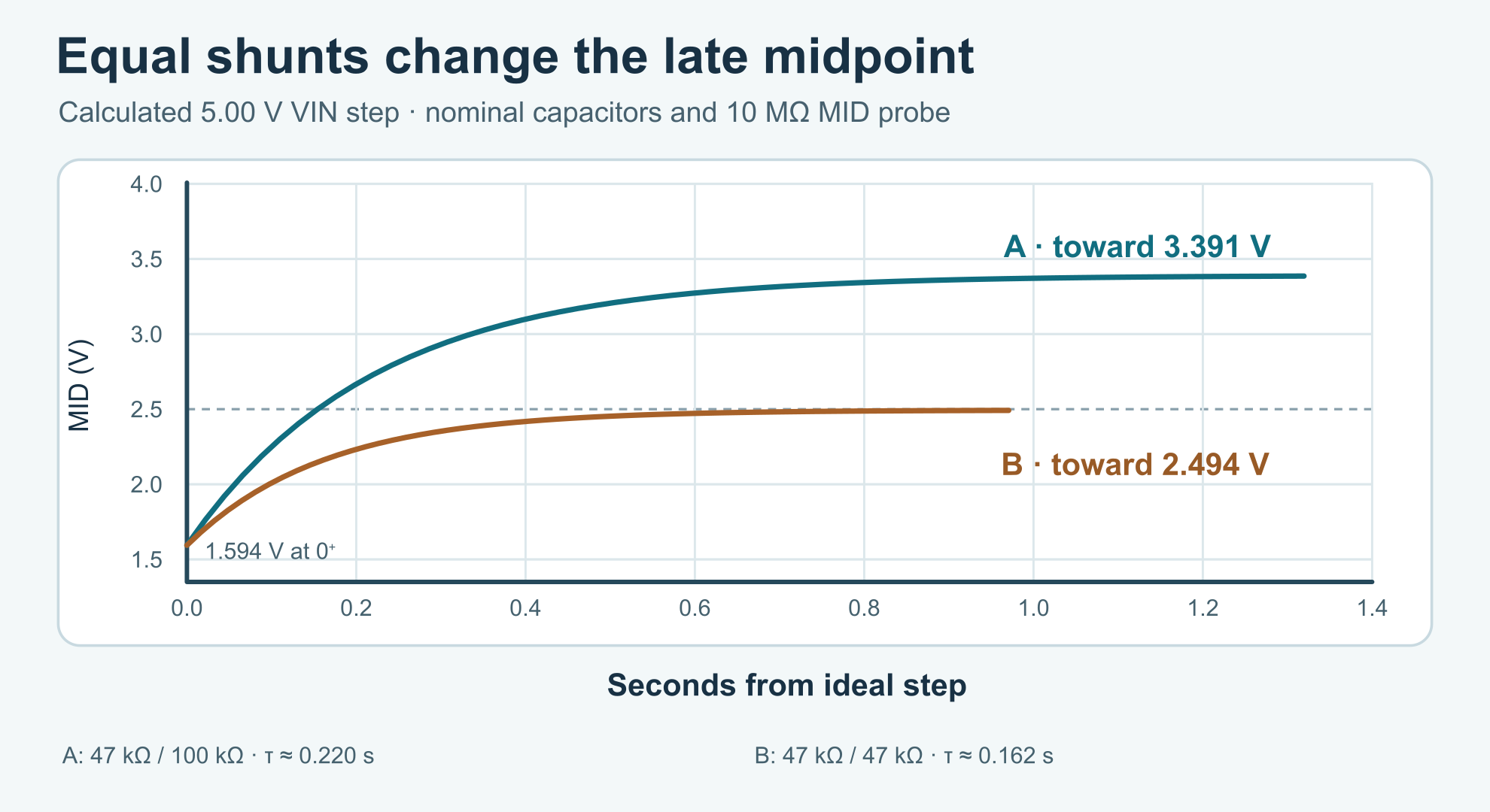
Immediately after an ideal step on VIN, the voltage redistribution is set by capacitance. With the fixture discharged, the fast change puts equal charge magnitudes on the two series capacitors. The larger capacitance needs less voltage for that charge. The midpoint jumps to VIN × C1 / (C1 + C2). The upper capacitor initially gets the remainder. For a 5.00 V ideal step, the midpoint is about 1.594 V and the upper capacitor gets about 3.406 V. An actual finite edge gives the resistors some time to act, so the first stable scope sample need not be exactly this value.
After settling, the ideal capacitors carry no steady current. The midpoint now follows the resistor divider. The 10 MΩ probe on MID is in parallel with R2. Call the total lower conductance Gb = 1/R2 + 1/Rprobe, where conductance is the reciprocal of resistance. Call the upper conductance Gt = 1/R1. The final midpoint is VIN × Gt / (Gt + Gb). At the nominal 5.00 V VIN and 10 MΩ probe, case A settles near 3.391 V and case B near 2.494 V. The 10 MΩ probe moves the nominal matched result down by about 6 mV. Ordinary resistor tolerances and the scope’s voltage accuracy can be larger than that shift. Treat it as a loading calculation unless your instrument can resolve it.
For a fixed VIN, the time constant is τ = (C1 + C2) / (Gt + Gb). A time constant describes how fast an exponential moves toward its final value. After one τ the midpoint has completed about 63.2% of its remaining change from the starting value. In A, τ is about 0.220 s. In B, it is about 0.162 s. VIN is held by a low-impedance source in this simplified calculation, which is why both capacitor terms are summed in the midpoint equation. The series capacitance seen by R3 during the fast edge is about 1.50 µF, giving a rough R3 time scale of 1.50 ms. It is much shorter than the two midpoint time constants.
For a varying VIN, Kirchhoff’s current law says current into the midpoint equals current out. The model gives (C1 + C2)·dMID/dt = C1·dVIN/dt + Gt·VIN − (Gt + Gb)·MID. The code integrates that equation exactly over each assumed linear segment between VIN samples. It ignores capacitor leakage, dielectric effects, probe capacitance and wire parasitics. Probe capacitance is tiny beside the 4.7 µF capacitor in this fixture. Keep the model’s simple scope separate from the actual errors of your bench.
tricky-circuit-campaigns133-138/batch-014/packages/series-capacitor-voltage-sharing/midpoint-step.svg).Capture two runs with the same capacitors
- Wire the fixture with the source disabled and S1 open. Check continuity to 0 V and identify both capacitor branches before powering up. Keep R1 and R2 in place. With S1 open, each capacitor can discharge through its own resistor. After any prior run, wait at least ten seconds and confirm that both MID and VIN minus MID are within 0.05 V of zero before the next capture.
- Install 100 kΩ at R2 for A. Measure both resistors out of circuit first if you want to put their measured values into the model. Arm a single trigger on the VIN rising edge near 2.5 V and close S1. Keep a discharged pretrigger interval and record at least 1.5 seconds after the rise. Use sample spacing of 0.2 ms or shorter through the edge, with both channels on the same time axis. Inspect VIN for bounce, clipping or a slow rise rather than assuming it was a clean ideal step.
- Record the actual late VIN and MID. Compare an early sample just after VIN rises with the ideal initial limit, and compare the stable tail with the resistor-divider estimate at the measured VIN. Use channel subtraction for C1 if available. Do not move a reference clip.
- Open S1, disable the supply and verify discharge before replacing R2 with 47 kΩ for B. Do not change the capacitors, probe settings or reference nodes. Repeat the capture. Use the worksheet (ZIP; file:
tricky-circuit-campaigns133-138/batch-014/packages/series-capacitor-voltage-sharing/observations-blank.csv) to keep the two runs, their actual values and the assumptions separate.
A large discrepancy can come from a swapped capacitor, an incorrect shunt, probe attenuation, a grounded MID, an unresolved supply edge, or the tolerance of the parts. Stop and inspect the wiring if a node is outside the expected 0–5 V range, the supply goes into current limit, or a part warms. Leave the supply disabled during changes. This small fixture teaches timing and voltage sharing. It supplies no high-voltage balancing design or qualification.
Run the complete analyzer
Save series_caps.py (ZIP; file: tricky-circuit-campaigns133-138/batch-014/packages/series-capacitor-voltage-sharing/series_caps.py) and run python3 series_caps.py for A, then python3 series_caps.py --bottom-kohm 47 for B. Python 3.9 or newer is sufficient. The ideal-step report includes both capacitor voltages, τ and 61 points from zero to six time constants. Add --probe-mohm 0 to see the model without that probe. Use actual resistance and capacitance values if you have suitable measurements.
For a capture, export comma-separated values (CSV) with the exact header time_s,source_v,midpoint_v. Use seconds and volts, one row per simultaneous observation and no unit suffix. The file must start near zero, finish with VIN at least 4.5 V and use ascending time. The program rejects gaps greater than 2 ms or shorter than 1 ns and limits the file to 50,000 rows. The 2 ms gate protects the model from very sparse data. It does not certify that the actual switching edge was resolved. The separate 0.2 ms procedure and scope view still matter.
To try that path with a known constructed input, download synthetic-capture.csv (ZIP; file: tricky-circuit-campaigns133-138/batch-014/packages/series-capacitor-voltage-sharing/synthetic-capture.csv) and run python3 series_caps.py --capture synthetic-capture.csv. With a real file, the report compares the recorded MID with the prediction driven by recorded VIN and gives the largest difference and its time. Its root mean square (RMS) error describes the typical magnitude of the residual, weighted equally by samples. It reports the final measured C1 and C2 voltages as well. This synthetic file was calculated using a 4 ms ramp and the same nominal circuit, so agreement verifies the arithmetic without validating the physical fixture.
"""Calculate series-capacitor sharing and compare a low-voltage capture."""

import argparse
import csv
import json
import math
from pathlib import Path


HEADER = ["time_s", "source_v", "midpoint_v"]


def bounded(value, low, high, label):
    if not math.isfinite(value) or not low <= value <= high:
        raise ValueError(f"{label} must be finite and between {low} and {high}")
    return value


def model(args):
    top = bounded(args.top_uf, .1, 50, "top capacitance") * 1e-6
    bottom = bounded(args.bottom_uf, .1, 50, "bottom capacitance") * 1e-6
    gt = 1 / (1000 * bounded(args.top_kohm, 1, 1000, "top resistance"))
    gb = 1 / (1000 * bounded(args.bottom_kohm, 1, 1000, "bottom resistance"))
    probe = bounded(args.probe_mohm, 0, 1000, "probe resistance")
    if 0 < probe < 1:
        raise ValueError("probe resistance must be at least 1 MΩ or zero for the unloaded model")
    if probe:
        gb += 1 / (probe * 1e6)
    return top / (top + bottom), gt / (gt + gb), (top + bottom) / (gt + gb)


def ideal_step(volts, alpha, beta, tau):
    first, final = alpha * volts, beta * volts
    samples = []
    for i in range(61):
        normalized = i / 10
        midpoint = final + (first - final) * math.exp(-normalized)
        samples.append({"t_over_tau": normalized, "time_s": normalized * tau,
                        "midpoint_v": midpoint, "top_v": volts - midpoint})
    return {"tau_s": tau, "initial_midpoint_v": first, "initial_top_v": volts - first,
            "final_midpoint_v": final, "final_top_v": volts - final, "samples": samples}


def read_capture(path):
    samples = []
    csv.field_size_limit(128)
    with path.open(encoding="utf-8-sig", newline="") as stream:
        reader = csv.reader(stream, strict=True)
        if next(reader, None) != HEADER:
            raise ValueError("CSV header must be " + ",".join(HEADER))
        for row in reader:
            if len(row) != 3 or len(samples) == 50_000:
                raise ValueError("expected three fields and at most 50,000 samples")
            try:
                t, source, midpoint = (float(text) for text in row)
            except ValueError as error:
                raise ValueError("CSV fields must be finite numbers") from error
            if not all(map(math.isfinite, (t, source, midpoint))):
                raise ValueError("CSV fields must be finite numbers")
            if abs(t) > 20 or not (-.1 <= source <= 5.5 and -.1 <= midpoint <= 5.5):
                raise ValueError("time or voltage outside the fixture range")
            if samples and not 1e-9 - 1e-14 <= t - samples[-1][0] <= .002 + 1e-12:
                raise ValueError("sample times must increase with gaps from 1 ns to 2 ms")
            samples.append((t, source, midpoint))
    if len(samples) < 3:
        raise ValueError("capture needs at least three samples")
    _, first_source, first_midpoint = samples[0]
    if max(abs(first_source), abs(first_midpoint), abs(first_source - first_midpoint)) > .05 + 1e-12:
        raise ValueError("capture must begin with the fixture discharged within 0.05 V")
    if samples[-1][1] < 4.5:
        raise ValueError("capture must finish high with at least 4.5 V at the source")
    return samples


def compare_capture(samples, alpha, beta, tau):
    previous_t, previous_v, predicted = samples[0]
    largest_gap = largest_error = error_sum = 0.0
    worst_time = previous_t
    for t, source, measured in samples[1:]:
        dt = t - previous_t
        h = dt / tau
        one_minus_decay = -math.expm1(-h)
        ramp_gain = one_minus_decay / h
        predicted += (beta * previous_v - predicted) * one_minus_decay
        predicted += (source - previous_v) * (beta + (alpha - beta) * ramp_gain)
        error = abs(measured - predicted)
        error_sum += error * error
        if error > largest_error:
            largest_error, worst_time = error, t
        largest_gap = max(largest_gap, dt)
        previous_t, previous_v = t, source
    return {
        "samples": len(samples), "largest_gap_ms": 1000 * largest_gap,
        "rms_error_v": math.sqrt(error_sum / len(samples)), "max_abs_error_v": largest_error,
        "max_error_time_s": worst_time, "last_predicted_midpoint_v": predicted,
        "last_measured_midpoint_v": samples[-1][2],
        "last_measured_top_v": samples[-1][1] - samples[-1][2],
    }


def main():
    parser = argparse.ArgumentParser(description=__doc__)
    parser.add_argument("--top-uf", type=float, default=2.2)
    parser.add_argument("--bottom-uf", type=float, default=4.7)
    parser.add_argument("--top-kohm", type=float, default=47)
    parser.add_argument("--bottom-kohm", type=float, default=100)
    parser.add_argument("--probe-mohm", type=float, default=10, help="0 means unloaded")
    parser.add_argument("--step-v", type=float, default=5, help="ideal reference step only")
    parser.add_argument("--capture", type=Path, help="optional aligned measured CSV")
    args = parser.parse_args()
    try:
        alpha, beta, tau = model(args)
        volts = bounded(args.step_v, 0, 5.5, "ideal step")
        report = {"capacitive_midpoint_ratio": alpha, "dc_midpoint_ratio": beta,
                  "ideal_step": ideal_step(volts, alpha, beta, tau)}
        if args.capture:
            report["capture"] = compare_capture(read_capture(args.capture), alpha, beta, tau)
    except (OSError, ValueError, csv.Error) as error:
        parser.exit(2, f"error: {error}\n")
    print(json.dumps(report, indent=2))


if __name__ == "__main__":
    main()
Challenge
In case B, what would change if you installed equal 4.7 µF capacitors but kept the two 47 kΩ resistors and the 10 MΩ probe? Which of the two midpoint limits would still differ from 2.500 V?
Check your reasoning
The initial capacitive ratio would become one half and the ideal initial midpoint would be 2.500 V. The lower probe still draws current, so the final midpoint would stay near 2.494 V. The larger sum of capacitances would lengthen τ by the factor 9.4/6.9. With unequal capacitors, matching the resistors only addresses the late divider.
Downloads and sources
The reader download (ZIP; file: tricky-circuit-campaigns133-138/batch-014/packages/series-capacitor-voltage-sharing/experiment-tests-v1.zip) includes the program, actual host tests, synthetic file, blank worksheet and original figures. Read the run notes (ZIP; file: tricky-circuit-campaigns133-138/batch-014/packages/series-capacitor-voltage-sharing/README-experiment.txt) for the two example commands. There are no collected bench results. The TLC555 one-shot experiment uses a charging capacitor to set a timer threshold. Here the two time regimes arise from a different network with two shunt paths.
- Vishay MKT1820, document 26011, film construction, 63 V order rows and terminal spacing. Vishay MKT1820 product information.
- Tektronix P2220 instructions, attenuation, input resistance, input capacitance and compensation.
Download the complete reader files (ZIP): full programs, blank observation worksheets, original editable SVG/PNG diagrams and selected support files for series-capacitor-voltage-sharing. Inline main programs remain complete; this download is supplementary.