A 10% duty-cycle pulse train (high for one-tenth of each period) can have a steady 0.600 V alternating component while its average voltage and the power it delivers to a resistor both change. Compare a bench multimeter in two voltage modes with the result of integrating an oscilloscope capture. A fixed resistor gives the three numbers a physical interpretation: only the total root mean square (RMS) voltage predicts its average electrical power.
Connect the three branches to one node
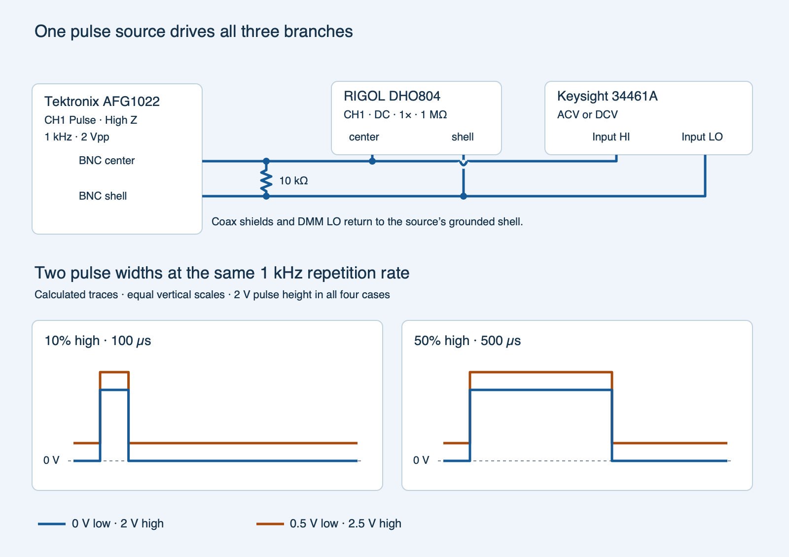
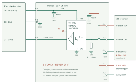
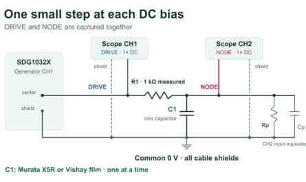
pulse-rms-fixture.svg)Use a Tektronix AFG1022 function generator, a RIGOL DHO804 oscilloscope, a Keysight 34461A digital multimeter (DMM), and one Vishay MRS25 10 kΩ ±1% axial resistor. Before connecting any input or output cables, connect the DHO804’s rear Ground Terminal to earth ground with its supplied ground cable, following the DHO800 User Guide. Its Type-C power input does not ground the instrument through the power cord. Use the supplied power adapter. Keep the AFG1022 and 34461A protective earth connections intact. Measure the loose resistor with the meter in resistance mode before wiring it. With the function generator output off, wire the resistor from the channel 1 (CH1) output center to its shell. From the same two nodes run a short coaxial branch into oscilloscope CH1 and a short pair to the 34461A’s front voltage Input HI and Input LO terminals. The shells, resistor return and Input LO join at the signal return. The line that bridges the return is a crossing without a connection. The shared signal return does not replace the DHO804’s required earth lead. Connect only the stated low-voltage bench generator.
Use a Bayonet Neill–Concelman (BNC) T adapter, a T-shaped three-way connector, and a short breakout at the junction. A coaxial cable has a center signal conductor surrounded by a conductive shield; BNC identifies its bayonet-style connector. Match the oscilloscope’s channel attenuation to the direct coaxial cable at 1×. Select direct-current (DC) coupling to retain the steady and changing parts of the signal, and use the 1 MΩ input. Keep 50 Ω termination off. The generator’s High Z (high-impedance) setting displays values for a very light assumed load. Its 50 Ω nominal output resistance still forms a divider with the 10 kΩ resistor. A 50 Ω source into 10 kΩ alone gives 10,000/(10,000 + 50) ≈ 0.995. The instruments add small loads, and the scope reading is the actual voltage across the resistor.
The maximum nominal instantaneous resistor power is 2.5 V squared divided by 10 kΩ, or 0.625 mW. The component dissipates much less than its 0.6 W rating throughout this fixture. Measure resistor voltage through the DMM’s voltage terminals only. A current or resistance setting would change the load and the meaning of the reading.
Change width, then raise both levels
- Set AFG1022 channel 1 to Pulse, 1 kHz and 2.00 V peak to peak (Vpp). Use 100 µs or 500 µs width. Those settings give 10% and 50% duty cycle, the fraction of each period spent high. A fixed square-wave preset can force 50% duty instead. Use the offset setting to target the low and high levels in the table. The displayed offset is the midpoint of the levels. For an asymmetric pulse it differs from the time average.
- Check both levels and capture the scope with DC coupling at a useful vertical range. A rising trigger near the observed midpoint and roughly a five-period record leave at least three complete rising-to-rising periods. Select 10 kpts for the Horizontal memory depth, then check that the actual exported interval is no greater than 2 µs. On the RIGOL open Storage → Save → Choose → Save Wave and choose Memory and CSV (comma-separated values). Save at least one record per mode. Preserve the calibrated CH1 voltage and the shared time origin. Keep the DMM connected during the captures.
- On the DMM choose DC voltage (DCV) with a fixed 10 V range, fixed 10 MΩ input, and at least 10 power line cycles of integration. A power line cycle is one cycle of the meter’s local mains reference. The long integration spans many pulses. Record three settled displayed voltages. Select alternating-current (AC) voltage (ACV), fixed 10 V range and the >20 Hz filter for the 1 kHz test. Wait at least one second after changing mode or signal, then take three settled readings. Leave the same meter leads in place. Check that switching modes did not visibly shift the scope levels, then label each capture and record the actual settings.
| Mode | High width | Low level | High level | Offset setting |
|---|---|---|---|---|
narrow_0 |
100 µs | 0 V | 2.0 V | +1.0 V |
narrow_up |
100 µs | 0.5 V | 2.5 V | +1.5 V |
half_0 |
500 µs | 0 V | 2.0 V | +1.0 V |
half_up |
500 µs | 0.5 V | 2.5 V | +1.5 V |
What each reading measures
For an ideal two-level pulse, let d be the duty fraction, L the low voltage and H the high voltage. Direct current (DC) refers here to the steady component or mean: VDC = (1 − d)L + dH. The total mean square weights the squares instead: Vtotal2 = (1 − d)L2 + dH2. The total RMS is its square root. Its unit is volts, and feeding a steady voltage of the same magnitude into a fixed resistor would deliver the same average power.
The alternating current (AC) component is the voltage variation around the mean. For the ideal pulse, its RMS is (H − L)√[d(1 − d)]. Shifting the low and high by the same amount leaves this variation unchanged. The total satisfies Vtotal2 = VDC2 + VAC2. The Keysight AC voltage function is AC-coupled, so its true RMS reading refers to the AC portion that falls inside the meter’s usable bandwidth. A pulse also contains harmonics, frequency components above its repetition rate. The 34461A manual discusses the meter’s finite 300 kHz AC voltage bandwidth and pulse-shape error. A 10% ideal pulse after subtracting its mean has a peak-to-RMS ratio (crest factor) of 1.8/0.6 = 3. Both the duty cycle and the actual waveform bandwidth matter.
For a fixed resistive load the predicted average electrical power is P = Vtotal2/R. The numbers below come from the ideal levels. The program calculates comparable quantities from actual scope samples. This test does not measure resistor temperature rise.
| Mode | DC mean | AC RMS | Total RMS | Power |
|---|---|---|---|---|
narrow_0 |
0.20 V | 0.60 V | 0.6325 V | 0.040 mW |
narrow_up |
0.70 V | 0.60 V | 0.9220 V | 0.085 mW |
half_0 |
1.00 V | 1.00 V | 1.4142 V | 0.200 mW |
half_up |
1.50 V | 1.00 V | 1.8028 V | 0.325 mW |
Compare the records
Put the scope samples in a CSV file with header mode,time_s,v. Enter seconds and volts, using rising timestamps within each mode. The blank meter worksheet (ZIP: meter-readings-blank.csv) has the required header mode,reading,vdc,vac_rms. Each mode needs three numbered readings from its two meter modes. Copy numeric values and strip instrument unit suffixes. Preserve the original exports and setting notes.
The analyzer finds 1 kHz periods and checks expected duty fractions, sample density and stable central plateaus. Between adjacent points it treats the signal as a linear segment. The mean-square contribution over duration Δt is Δt(a2 + ab + b2)/3. It averages the normalized moments over the complete stable periods with equal weight for each cycle. The scope AC RMS and total RMS are then calculated from those moments. For each meter mode, the median is the middle of its three sorted readings. The two meter medians are compared with the corresponding scope quantities. Within each width it asks the mean to shift by approximately 0.50 V while the AC-only RMS remains similar. The allowed millivolt differences are procedural, not instrument accuracy tolerances.
Run python3 pulse_rms.py scope.csv meter.csv --resistance-ohm 10000 and replace 10000 with the measured resistance in ohms. Omitting the option uses the nominal value. Exit 0 reports supported values. Exit 1 marks an unresolved result from FixtureError, including wrong headers, invalid fields or modes, nonnumeric or out-of-range values, time/order or missing-mode errors, and failed fixture or comparison checks. Exit 2 reports file-access, text-decoding or CSV-syntax errors; argument-parser errors also exit 2. The results table is printed only after all four modes pass. If the two instruments disagree, check input range and coupling, the meter mode, the sample interval and whether the waveform or meter settled. The script checks numerical consistency under the recorded setup. It does not verify entered meter settings or calibration. Report the observed disagreement if the measurements fail the checks.
Predict a new offset
Keep the same 10% duty and 2 V pulse height. If you set the low level to 1 V and the high level to 3 V, what are the three ideal readings and the predicted power in 10 kΩ?
Answer
The mean is 1.20 V, the AC RMS is still 0.60 V, and the total RMS is √(1.20² + 0.60²) ≈ 1.342 V. The average power is 1.80/10,000 W = 0.180 mW. This is an algebra exercise outside the analyzer’s four fixture modes.
Full Python analyzer
Download the standalone code (ZIP: pulse_rms.py) or use the experiment archive (ZIP: experiment-tests-v1.zip) with diagram, blank worksheet and tests. The archive contains two files beginning with synthetic- so you can try the analyzer before connecting equipment. The tests and those files use calculated data. Fill the observation worksheet from your own instruments.
Complete source for pulse_rms.py
#!/usr/bin/env python3
"""Separate the mean, AC-only RMS and total RMS of a 1 kHz pulse experiment."""

import argparse
import csv
import math
from pathlib import Path
from statistics import median
import sys


MODES = {"narrow_0": (0.10, 0), "narrow_up": (0.10, 0.50),
         "half_0": (0.50, 0), "half_up": (0.50, 0.50)}


class FixtureError(ValueError):
    """The four records do not establish the comparison."""


def check(ok, mode, message):
    if not ok:
        raise FixtureError(f"{mode}: {message}")


def rows(path, header, limit):
    with Path(path).open(newline="", encoding="utf-8-sig") as stream:
        reader = csv.reader(stream, strict=True)
        check(tuple(next(reader, [])) == header, path, "unexpected CSV header")
        for n, row in enumerate(reader, 2):
            check(n <= limit + 1 and len(row) == len(header) and row[0] in MODES,
                  path, f"unexpected row at line {n}")
            try:
                values = tuple(map(float, row[1:]))
            except ValueError as exc:
                raise FixtureError(f"{path}: nonnumeric value at line {n}") from exc
            check(all(math.isfinite(v) for v in values), path, f"non-finite value at line {n}")
            yield row[0], values


def load_files(wave_path, meter_path):
    wave = {mode: [] for mode in MODES}
    meter = {mode: {} for mode in MODES}
    for mode, pair in rows(wave_path, ("mode", "time_s", "v"), 100_000):
        wave[mode].append(pair)
    for mode, (index, dc, ac) in rows(meter_path, ("mode", "reading", "vdc", "vac_rms"), 12):
        check(index in (1, 2, 3) and index not in meter[mode],
              mode, "meter needs unique readings numbered 1–3")
        meter[mode][index] = (dc, ac)
    return wave, {mode: list(group.values()) for mode, group in meter.items()}


def interval_moments(points):
    duration = points[-1][0] - points[0][0]
    area = squared = 0.0
    for (t1, a), (t2, b) in zip(points, points[1:]):
        dt = t2 - t1
        area += dt * (a + b) / 2
        squared += dt * (a*a + a*b + b*b) / 3
    return area / duration, squared / duration


def scope_moments(wave, mode, expected_duty, low):
    check(bool(wave), mode, "no scope samples")
    for t, v in wave:
        check(math.isfinite(t) and math.isfinite(v) and abs(t) <= 10 and -0.20 <= v <= 2.75,
              mode, "sample or plateau outside fixture envelope")
    edges = []
    threshold = low + 1
    for i, ((left_t, left_v), (right_t, right_v)) in enumerate(zip(wave, wave[1:]), 1):
        check(0 < right_t - left_t <= 2.0e-6 + 1e-12, mode,
              "sample gap must be positive and no larger than 2 us")
        if (left_v >= threshold) != (right_v >= threshold):
            fraction = (threshold - left_v) / (right_v - left_v)
            edges.append((i, left_t + fraction * (right_t - left_t), right_v >= threshold))
    rises = [i for i, (_, _, rising) in enumerate(edges) if rising]
    check(len(rises) >= 4, mode, "need at least three complete high–low periods")
    period_means, period_squares = [], []
    for first, last in zip(rises, rises[1:]):
        check(last == first + 2, mode, "unexpected edge sequence")
        start_index, start, _ = edges[first]
        fall_index, fall, _ = edges[first + 1]
        stop_index, stop, _ = edges[last]
        period = stop - start
        on_time = fall - start
        check(.00098 <= period <= .00102, mode, "pulse frequency differs from 1 kHz")
        check(abs(on_time / period - expected_duty) <= .015, mode,
              "duty cycle differs from selected mode")
        high_samples = [
            v for t, v in wave[start_index:fall_index]
            if start + .2 * on_time <= t <= start + .8 * on_time
        ]
        tail_time = stop - fall
        low_samples = [
            v for t, v in wave[fall_index:stop_index]
            if fall + .2 * tail_time <= t <= fall + .8 * tail_time
        ]
        for samples, target in ((high_samples, low + 2), (low_samples, low)):
            check(len(samples) >= 15 and abs(median(samples) - target) <= .065
                  and max(samples) - min(samples) <= .070, mode,
                  "plateau level or stability differs from target")
        points = [(start, threshold), *wave[start_index:stop_index], (stop, threshold)]
        mean, square = interval_moments(points)
        period_means.append(mean)
        period_squares.append(square)
    check(max(period_means) - min(period_means) <= .025 and
          max(period_squares) - min(period_squares) <= .060, mode,
          "period moments vary too much")
    return sum(period_means) / len(period_means), sum(period_squares) / len(period_squares)


def analyze(wave, meter, resistance_ohm):
    check(math.isfinite(resistance_ohm) and 9700 <= resistance_ohm <= 10300,
          "fixture", "resistance must be measured near the nominal 10 kohm")
    results = {}
    for mode, (duty, low) in MODES.items():
        mean, squared = scope_moments(wave[mode], mode, duty, low)
        total = math.sqrt(squared)
        ac = math.sqrt(max(0.0, squared - mean * mean))
        check(len(meter[mode]) == 3, mode, "need three paired meter readings")
        dc_values, ac_values = zip(*meter[mode])
        for values in (dc_values, ac_values):
            check(all(math.isfinite(v) and 0 <= v <= 3 for v in values), mode,
                  "meter reading outside fixture envelope")
            check(max(values) - min(values) <= .025, mode, "meter reading spread too large")
        meter_dc, meter_ac = median(dc_values), median(ac_values)
        check(abs(meter_dc - mean) <= .055, mode, "DC meter and scope mean disagree")
        check(abs(meter_ac - ac) <= .055, mode, "AC meter and scope AC-only RMS disagree")
        results[mode] = {"mean": mean, "ac": ac, "total": total, "meter_dc": meter_dc,
                         "meter_ac": meter_ac, "power_mw": 1000 * squared / resistance_ohm}
    for prefix in ("narrow", "half"):
        base, shifted = (results[f"{prefix}_{suffix}"] for suffix in ("0", "up"))
        check(.43 <= shifted["mean"] - base["mean"] <= .57, prefix,
              "scope did not verify the 0.50 V offset change")
        check(abs(shifted["ac"] - base["ac"]) <= .045 and
              abs(shifted["meter_ac"] - base["meter_ac"]) <= .050, prefix,
              "AC-only RMS varied across the offset pair")
    return results


def main(argv=None):
    parser = argparse.ArgumentParser(description=__doc__)
    parser.add_argument("scope_csv")
    parser.add_argument("meter_csv")
    parser.add_argument("--resistance-ohm", type=float, default=10_000,
                        help="measured load in ohms; default nominal 10000")
    args = parser.parse_args(argv)
    try:
        wave, meter = load_files(args.scope_csv, args.meter_csv)
        results = analyze(wave, meter, args.resistance_ohm)
    except (OSError, UnicodeError, csv.Error) as exc:
        print(f"ERROR: {exc}", file=sys.stderr)
        return 2
    except FixtureError as exc:
        print(f"UNRESOLVED: {exc}", file=sys.stderr)
        return 1
    print("mode         scope DC   scope AC   scope total     DMM DC    DMM AC   load mW")
    for mode, item in results.items():
        print(f"{mode:11} {item['mean']:9.4f} {item['ac']:10.4f} {item['total']:12.4f} "
              f"{item['meter_dc']:10.4f} {item['meter_ac']:9.4f} {item['power_mw']:9.4f}")
    if args.resistance_ohm == 10_000:
        print("Power uses 10000 ohms; check the actual resistor.")
    return 0


if __name__ == "__main__":
    sys.exit(main())
Related reading and primary sources
- Pulse-width modulation lesson introduces how duty fraction changes the average. The AFG1022 load-display experiment explains why the generator’s load setting is separate from the real load.
- Tektronix AFG1000 Series datasheet for AFG1022 Pulse settings, load display and nominal output impedance.
- Keysight Truevolt Operating and Service Guide for 34461A voltage modes and AC pulse-shape error in the Measurement Tutorial.
- RIGOL DHO800 Series datasheet for the DHO804 input specifications and user guide for direct channel settings, memory depth and CSV wave export.
- Vishay MRS16/MRS25 datasheet for the 10 kΩ resistor’s family, tolerance and power rating.
Download the complete reader files (ZIP) for the original editable drawing, PNG, worksheet and code in pulse-train-dc-ac-rms-heating. The full main program is also included above.